Max cut¶

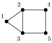
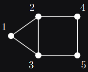
Consider the following undirected graph with 5 nodes

The semidefinite approximation of the max cut problem [1] corresponding to this graph is

\[ \begin{align}\begin{aligned}\max_{X \in \mathbb{S}^5} &&& \langle C, X \rangle\\\text{subj. to} &&& X_{ii} = 1 \qquad i=1,\ldots,5\\&&& X \succeq 0,\end{aligned}\end{align} \]

where

\[\begin{split}C = \begin{bmatrix} 2 & -1 & -1 & 0 & 0 \\ -1 & 3 & -1 & -1 & 0 \\ -1 & -1 & 3 & 0 & -1 \\ 0 & -1 & 0 & 2 & -1 \\ 0 & 0 & -1 & -1 & 2 \end{bmatrix}.\end{split}\]

We show how we can solve this semidefinite program using QICS below.

import numpy as np

import qics

# Define objective function
C = numpy.array([
    [ 2., -1., -1.,  0.,  0.],
    [-1.,  3., -1., -1.,  0.],
    [-1., -1.,  3.,  0., -1.],
    [ 0., -1.,  0.,  2., -1.],
    [ 0.,  0., -1., -1.,  2.]
])
c = -qics.vectorize.mat_to_vec(C)

# Build linear constraint
A = np.zeros((5, 25))
A[np.arange(5), np.arange(0, 25, 6)] = 1.

b = np.ones((5, 1))

# Define cones to optimize over
cones = [qics.cones.PosSemidefinite(5)]

# Initialize model and solver objects
model  = qics.Model(c=c, A=A, b=b, cones=cones)
solver = qics.Solver(model, verbose=0)

# Solve problem
info = solver.solve()

X_opt = info["s_opt"][0][0]
print("Optimal matrix variable X is:")
print(X_opt)
print("which has rank:", np.linalg.matrix_rank(X_opt, tol=1e-6))

Optimal matrix variable X is:
[[ 1.         -0.36684149 -0.3668415   0.12486877  0.12486877]
 [-0.36684149  1.         -0.73085463 -0.96880942  0.87719533]
 [-0.3668415  -0.73085463  1.          0.87719533 -0.96880942]
 [ 0.12486877 -0.96880942  0.87719533  1.         -0.96881558]
 [ 0.12486877  0.87719533 -0.96880942 -0.96881558  1.        ]]
which has rank: 2

Complex max cut¶

In signal processing [2], the following complex variation of the semidefinite relaxation of max cut arises

\[ \begin{align}\begin{aligned}\min_{X \in \mathbb{H}^n} &&& \langle C, X \rangle\\\text{subj. to} &&& X_{ii} = 1 \qquad i=1,\ldots,5\\&&& X \succeq 0,\end{aligned}\end{align} \]

where

\[C = \text{diag}(v)(\mathbb{I} - UU^\dagger)\text{diag}(v)\]

for some complex matrix \(U \in \mathbb{C}^{n \times m}\) and real vector \(v \in \mathbb{R}^n\). We can solve this in QICS by making a few adjustments to the previous code.

import numpy as np

import qics

np.random.seed(1)

n = 5
m = 4
vn = qics.vectorize.vec_dim(n, iscomplex=True)

# Generate random linear objective function
U = np.random.randn(n, m) + np.random.randn(n, m)*1j
v = np.random.randn(n)
C = np.diag(v) @ (np.eye(n) - U @ U.conj().T) @ np.diag(v)
c = qics.vectorize.mat_to_vec(C)

# Build linear constraints  Xii = 1 for all i
A = np.zeros((n, vn))
A[np.arange(n), np.arange(0, vn, 2 * n + 2)] = 1.

b = np.ones((n, 1))

# Define cones to optimize over
cones = [qics.cones.PosSemidefinite(n, iscomplex=True)]

# Initialize model and solver objects
model  = qics.Model(c=c, A=A, b=b, cones=cones)
solver = qics.Solver(model)

# Solve problem
info = solver.solve()

X_opt = info["s_opt"][0][0]
print("Optimal matrix variable X is: ")
print(np.round(X_opt, 3))
print("which has rank:", np.linalg.matrix_rank(X_opt, tol=1e-6))

Optimal matrix variable X is:
[[ 1.   +0.j     0.209-0.978j  0.67 -0.743j -0.584+0.812j  0.866-0.499j]
 [ 0.209+0.978j  1.   +0.j     0.866+0.499j -0.916-0.401j  0.67 +0.743j]
 [ 0.67 +0.743j  0.866-0.499j  1.   +0.j    -0.994+0.11j   0.951+0.309j]
 [-0.584-0.812j -0.916+0.401j -0.994-0.11j   1.   +0.j    -0.911-0.412j]
 [ 0.866+0.499j  0.67 -0.743j  0.951-0.309j -0.911+0.412j  1.   +0.j   ]]
which has rank: 1

References¶

“Improved approximation algorithms for maximum cut and satisfiability problems using semidefinite programming,” M. X. Goemans, and D. P. Williamson, Journal of the ACM (JACM) 42.6 (1995): 1115-1145.

“Phase recovery, maxcut and complex semidefinite programming”, I. Waldspurger, A. d’Aspremont, and S. Mallat. Mathematical Programming, pp. 1-35, 2012.